Download These Notes

Notes of Advance Algorithm Analysis and Design

Prepared by Ambreen Sarwar

Introduction to algorithms

Algorithms

An algorithm is a tool for solving a given problem. An algorithm is the finite sequence of instructions such that each instruction is

1. Well define and clear meaning
2. Give output in finite amount of time
3. Can be performed easily

An algorithm has the following criteria:

Input: The algorithm must have input values from the specified set.

Output:Each algorithm is written to produce the output. So, the algorithm must give output on given set of input values.

Definiteness:Every algorithm must be well define and has clear meaning.

Finiteness: Every algorithm must be terminating after finite steps.

Effectiveness:Every algorithm is effective which performs some specific action on the given data.

Efficient: Algorithm should be efficient. It should not useunnecessary memory location.

Concise and compact: Algorithm should be concise and compact.

Factors affecting the speed of algorithm

There are following factor that affect the speed of algorithm:

Number of input:

The number of input values can affect the speed of algorithm. For example if we use 100 as a input value, it take lot of time as compare to if we use 10 as a input value. So, there is different speed on different input values.

Processor speed:

The speed of algorithm is also affected by the processor speed. For example the speed of processor is slow then the speed of algorithm is also slow and if the speed of processor is high then it can increase the speed of algorithm.

Simultaneous programs:

The speed of algorithm is also affected by the simultaneous programs. It means that if more than one programs are execute then they directly affect the speed of program because processor becomes busy to execute every program.

Location of items:

The location of items affects the speed. For example, an item is located in memory on 5thposition; it takes less time to access as compare to an item located on 1000th position.

Different implementations:

Different softwares are also affecting the speed. For example, speed of a program is different on window XP operating system and on window8 operating system.

Algorithm analysis

Algorithm analysis is to study the efficiency of algorithms when the input size grow, based on the number of steps, the amount of computer time and space. We can measure the performance of an algorithm by computing following factors:

1. Time complexity

2. Space complexity

3. Measuring an input size

4. Measuring running time

5. Order of growth

6. Best case, worst case and average case analysis

Space complexity:

The space complexity can be defined as amount of memory required by an algorithm to run.

To compute the space complexity we use two factors: constant and instance characteristics. The space requirement S(p) can be given as:

S(p) = C + Sp

Where C is the constant i.e. fixed part and it denotes the space of inputs and outputs. This space is an amount of space taken by instruction, variables and identifiers. And Sp is a space dependent upon instance characteristics. This is a variable part whose space requirement depends on particular problem instance.

Time complexity:

The space complexity can be defined as amount of computer time required by an algorithm to run to completion.

The time complexity dependent on following factors:

1. System load

2. Number of other programs running

3. Instruction set used

4. Speed of underlying hardware

The time complexity is therefore given in terms of frequency count. Frequency count is a count denoting number of times of execution of statement.

Measuring an input size:

It is observed that if the input is longer, then algorithm runs for a longer time. Hence we can compute the efficiency of an algorithm as a function to which input size is passed as a parameter. Sometimes to implement an algorithm we require prior knowledge of input size.

Measuring running time:

1. We have already studied that the time complexity is measured in terms of a unit called frequency count.The time which is measured for analyzing an algorithm is generally running time.
2. First we identify the important operation of the algorithm. This operation is called the basic operation.
3. It is not difficult to identify the basic operation from an algorithm. Generally the operation which is more time consuming is the basic operation of the algorithm. Normally such basic operation is located in inner loop.
4. Then we compute the total number of time taken by this basic operation. We can compute the running time by using the following formula:

n	log n	n log n	n2	2n
1	0	0	1	2
2	1	2	4	4
4	2	8	16	16
8	3	24	64	256
16	4	64	256	65,536
32	5	160	1024	4,294,967,296

Best case, worst case and average case analysis:

If an algorithm takes minimum amount of time to run to completion for a specific set of input then it is called best case time complexity.

If an algorithm takes maximum amount of time to run to completion for a specific set of input then it is called worst case time complexity.

The time complexity that we get from certain set of inputs is as an average same. Therefore, corresponding input such a time complexity is called average case time complexity.

Growth of Functions

To choose the best algorithm, we need to check the efficiency of each algorithm. The efficiency can be measured by computing the time complexity of each algorithm. Asymptotic notation is a shorthand way to represent the time complexity.

Various notations such as Ω, θ, O used are called asymptotic notations.

Big oh notation

The big oh notation is denoted by "O". it is the method of representing the upper bound of algorithm's running time. Using big oh notation we can give longest amount of time taken by the algorithm to complete.

Let f(n) and g(n) be non-negative functions. Let n_o and constant c are two integers such that n_o denotes some value of input and n>n_o.

Similarly c is some constant such that c>0. We can write

F(n) ≤ c * g(n)

F(n) is the big oh of g(n). it is also denoted as f(n) є O(g(n)). In other words f(n) is less than g(n) if g(n) is multiple of some constant c.

Consider function f(n) = 2n+2 and g(n) = n^2. We have to find some constant c, so that F(n) ≤ c * g(n).

As f(n) = 2n+2 and g(n) = n² then we find c for n = 1

f(n) = 2n+2

f(1) = 2(1)+2

f(1) = 4

and

g(n) = n²

g(1) = 1²

g(1) = 1

i.e. f(n) > g(n)

If n = 2 then,

f(n) = 2n+2

f(2) = 2(2)+2

f(1) = 6

and

g(n) = n²

g(2) = 2²

g(2) = 4

i.e. f(n) > g(n)

If n = 3 then,

f(n) = 2n+2

f(3) = 2(3)+2

f(1) = 8

and

g(n) = n²

g(3) = 3²

g(3) = 9

i.e. f(n) < g(n) is true

Hence we can conclude that for n>2, we obtain

f(n) < g(n)

h2 class="myh1">Omega notation

The omega notation is denoted by "Ω". It is the method of representing the lower bound of algorithm's running time. Using omega notation we can give shortest amount of time taken by the algorithm to complete.

The function f(n) is said to be in Ω(g(n)) if f(n) is bounded below by some positive constant multiple of g(n) such that

F(n) ≥ c * g(n) for all n ≥n_o

F(n) is the omega of g(n). it is also denoted as f(n) є Ω(g(n)). Graphically we can represent it as:

Consider function f(n) = 2n²+2 and g(n) = 7n. We have to find some constant c, so that F(n) ≥ c * g(n).

As f(n) = 2n²+2 and g(n) = 7n then we find c for n = 1

f(n) = 2n²+2

f(1) = 2(1)²+2

f(1) = 4

and

g(n) = 7n

g(1) = 7(1)

g(1) = 7

i.e. f(n) < g(n)

If n = 2 then,

f(n) = 2n²+2

f(2) = 2(2)²+2

f(2) = 10

and

g(n) = 7n

g(2) = 7(2)

g(2) = 14

i.e. f(n) < g(n)

If n = 3 then,

f(n) = 2n²+2

f(3) = 2(3)²+2

f(3) = 20

and

g(n) = 7n

g(3) = 7(3)

g(3) = 21

i.e. f(n) < g(n)

If n = 4 then,

f(n) = 2n²+2

f(4) = 2(4)²+2

f(4) = 34

and

g(n) = 7n

g(4) = 7(4)

g(4) = 28

i.e. f(n) > g(n) is true

Hence we can conclude that for n>3, we obtain

f(n) > g(n)

Theta notation:

The theta notation is denoted by 'θ'. By this method the running time is between lower and upper bound.

Let f(n) and g(n) be non-negative functions. There are two positive constants namely c₁ and c₂. Such that

c1 * g(n) ≤ f(n) ≤ c₂ * g(n)

It is also denoted as f(n) є θ(g(n)).

Mathematicalanalysis of non-recursive algorithm:

Mathematicalanalysis of non-recursive algorithm

First of all we will see the general plan for analyzing the efficiency of non-recursive algorithms. This plan tells us the steps to be followed while analyzing such algorithms.

General plan:

1. Decide the input size based on parameter n.

2.   Identify the basic operation of the algorithm.

3.   Check how many times the basic operation is executed. Then find whether the execution of basic operation depends upon the input size n. Determine the worst, average and best cases for input of size n. if the basic operation depends upon the worst case, average case and best case then that has to be analyzed separately.

4. Set up a sumfor the number of times the basic operation is executed.

5. Simplify the summation using the standard formula and rules.

Summation formulas and rules

There are seven rules which are as follow:

Where n and k are some upper and lower limits
Mathematical analysis of recursive algorithm:
            First of all we will see the general plan for analyzing the efficiency of recursive algorithms. This plan tells us the steps to be followed while analyzing such algorithms.
General plan:
  Decide the input size based on parameter n.
  Identify the basic operation of the algorithm.
  Check how many times the basic operation is executed. Then find whether the execution of basic operation depends upon the input size n. Determine the worst, average and best cases for input of size n. if the basic operation depends upon the worst case, average case and best case then that has to be analyzed separately.
Set up a recurrence relation with some initial condition and expressing the basic operation.
 Solve the recurrence or at least determine the order of growth. While solving the recurrence we will use the forward and backward substitution method. And then correctness of formula can be proved with the help of mathematical induction method.
Example:

Solve the following recurrence relations:

a. x(n) = x(n - 1) + 5 for n > 1, x(1) = 0

b. x(n) = x(n/2) + n for n > 1, x(1) = 1(solve for n = 2^k)

a. x(n) = x(n - 1) + 5 for n > 1, x(1) = 0

x(n) = x(n - 1) + 5

x(n) = [x(n - 2) + 5] +5

x(n) = [x(n - 3) + 5] +5 +5

x(n) = x(n - 3) + 5 * 3

x(n) = x(n - i) + 5 * i

if i = n -1 then

x(n) = x(n - i) + 5 * i

x(n) = x(n -(n - 1)) + 5 * (n - 1)

x(n) = x(n -n + 1) + 5 * (n - 1)

x(n) = x(1) + 5 * (n - 1)

x(n) = 0 + 5 * (n - 1)

x(n) = 5 * (n - 1)

b.x(n) = x(n/2) + n for n > 1, x(1) = 1(solve for n = 2^k)

x(n) = x(n/2) + n

x(2^k) = x(2^k /2) + 2^k

x(2^k) = x(2^k - 1) + 2^k

x(2^k) = [x(2^k-2 ) + 2^k-1] + 2^k

x(2^k) = x(2^k-3) + 2^k-2 + 2^k-1 + 2^k

x(2k) = x(2k- i) + 2k- i +1 + 2k- i +2 +....+ 2k

if i = k then

x(2k) = x(2k-k) + 2k- k +1 + 2k- k +2 +........+ 2k

x(2k) = x(20) + 21 + 22 +.....+ 2k

x(2k) = x(1) + 21 + 22 +.......+ 2k

x(2k) = 1 + 21 + 22 +......+ 2k

x(2k) = 2k + 1 - 1

x(2k) = 2.2k - 1

x(2k) = 2.n - 1

 

Empirical analysis of algorithms

We have discussed the mathematical analysis of algorithms for both recursive and non recursive algorithms. The analysis of algorithms can be done in two ways:

• Mathematical analysis
•  Empirical analysis

We have already discussed the mathematical analysis. We can analyze an algorithm by another method called empirical analysis. Empirical analysis of algorithm means observing behaviour of an algorithm for certain set of input. In empirical analysis actual program is written for the corresponding algorithm and with the help of some suitable input set, the algorithm is analyzed. Let us discuss the steps to be followed while analyzing algorithm empirically.

General plan for empirical analysis

1. Understand the purpose of experiment of given algorithm.

2. Decide the efficiency metric M. also decide the measurement unit. For example operation's count Vs time.

3. Decide on characteristics of the input.

4. Create a program for implementing the algorithm. This program is ready for experiment.

5. Generate a sample of input.

6. Run the algorithm for some set of input sample. Record the results obtained.

7. Analyze the resultant data.

Chapter 2

Divide and conquer

Introduction:

In divide and conquer strategy the problem is broken down into two sub problems and solution to these sub problems is obtained.

General method:

In divide and conquer method, a given problem is,

• Divided into smaller sub problems
• These problems are solved independently
• Combining all the solutions of the sub problems into solution of the whole.

If the sub problems are large enough then divide and conquer is reapplied. The generated sub problems are usually of same type as the original problem. Hence recursive algorithms are in divided and conquer strategy.

Binary search

Binary search is an efficient searching method. While searching the elements using this method the most essential thing is that the elements in the array should be sorted one.

An element which is to be searched from the list of elements stored in array A[0.......n -1] is called KEY element.

Let A[m] be the mid element of array A. Then there are three conditions that need to be tested while searching the array using this method.

1. If KEY = A[m] then desired element is present in the list.

2. Otherwise if KEY < A[m] then search the left sub list.

3. Otherwise if KEY > A[m] then search the right sub list.

Example:

Consider a list of elements stored in array A as

 

0	1	2	3	4	5	6
10	20	30	40	50	60	70
Low						High

The KEY element (the element to be searched) is 60. Now to obtain middle element we will apply a formula:

m = (low + high)/2

m = (0 + 6)/2

m = 3

Then check A[m] = KEY, but A[3] = 40 which is less than 60. So, search is take place at right side of the mid.

A[m] = KEY

A[5] = 60

The number is present in the list. Thus, we can search the desired number from the list of elements.

Analysis:

The basic operation in binary search is comparison of search key with the array elements. To analyze efficiency of binary search we count the number of times the search key gets compared with the array elements. The comparison is also called a three way comparison because algorithm makes the comparison to determine whether KEY is smaller, equal to or greater than a[m].

In the algorithm after one comparison the list of n elements is divided into n/2 sublists. The worst case efficiency is that the algorithm compares all the array elements for searching the desired element. In this method one comparison is made and based on this comparison array is divided each time in n/2 sublists. Hence the worst case time complexity is given by:

C_worst(n) = C_worst(n/2) + 1 for n > 1

Where

Cworst(n/2) is the time required to compare left sublist or right sublist. 1 is the one comparison made with middle element.

 

Also, Cworst(1) = 1

But as we consider the rounded down value when array gets divided the above equation can be written as

Cworst(n) = Cworst(n/2) + 1 for n > 1 .....(1)

Cworst(1) = 1....(2)

The above recurrence relation can be solved further. Assume n = 2k the equation (1) becomes,

C_worst(2^k) = C_worst(2^k/2) + 1

C_worst(2^k) = C_worst(2^{k - 1}) + 1 .....(3)

Using backward substitution method, we can substitute

C_worst(2^{k - 1}) = C_worst(2^{k - 2}) + 1

Then equation (3) becomes

C_worst(2^k) = [C_worst(2^{k - 2}) + 1] + 1

C_worst(2k) = C_worst(2^{k - 2}) + 2

Then

C_worst(2^k) = [C_worst(2^{k - 3}) + 1] + 2

C_worst(2^k) = C_worst(2^{k - 3}) + 3

----

----

C_worst(2^k) = C_worst(2^{k - k}) + k

C_worst(2^k) = C_worst(2⁰) + k

C_worst(2^k) = C_worst(1) + k .....(4)

But as per equation(2)

Cworst(1) = 1

Putting in equation (4) we get

C_worst(2k) = 1 + k .....(5)

As we have assumed

n = 2k

taking logarithm (base 2) on both sides

log² n = log₂ 2^k

log² n = k log₂ 2

log² n = k (1)

log² n = k

Putting the value of k in equation (5) we get

C_worst(n) = 1 + log₂ n

C_worst(n) ≈ log₂ n for n > 1

The worst case time complexity of binary search is θ(log₂ n).

Average case:

To obtained average case efficiency of binary search we will consider some samples of input n.

If n = 1, where the search KEY = 11

0

11

 

In this case there is only one comparison required to search KEY.

If n = 2, where the search KEY = 22

0	11
1	22

 In this case there are two comparisons required to search KEY.

If n = 4, where the search KEY = 44

0	11
1	22
2	33
3	44

In this case there are three comparisons required to search KEY. Because

m = (low + high)/2

m = (0 + 3)/2

m = 1

As A[1] = 22 and 22< 44. Search right sublist, again

m = (low + high)/2

m = (2 + 3)/2

m = 2

As A[2] = 33 and 33< 44. Search right sublist, again

m = (low + high)/2

m = (3 + 3)/2

m = 3

As A[3] = 44. Similarly so on.

Observing the above process we can write

log₂ n + 1 = c

for instance if n = 2 then

log₂ 2 + 1 = c

1 + 1 = c

2 = c

Similarly if n = 8, then

log₂ n + 1 = c

log₂ 8 + 1 = c

3 + 1 = c

4 = c

Thus, we can write that, average case time complexity of binary search is θ(log₂ n).

 

Time complexity of binary search

Best case	Average case	Worst case
θ(1)	θ(log2 n)	θ(log2 n)

Merge sort

The merge sort is a sorting algorithm that uses the divide and conquer strategy. In this method division is dynamically carried out.

Merge sort on an input array with n elements consists of three steps:

Divide: partition array into two sub lists s1 and s2 with n/2 elements each.

Conquer: then sort sub list s1 and sub list s2.

Combine: merge s1 and s2 into a unique sorted group.

Example:

Consider the elements as

70, 20, 30, 40, 10, 50, 60

Now we will split this list into two sublists.

Analysis

In merge sort algorithm the two recursive calls are made. Each recursive call focuses on n/2 elements of the list. After two recursive calls one call is made to combine two sublists i.e. to merge all n elements. Hence we can write recurrence relation as:

T(n) = T(n/2) + T(n/2) + cn

Where, n > 1 and T(1) = 0

T(n/2) is the time taken by left or right sublist to get sorted. And the cn is the time taken for combining two sublists.

We can obtain the time complexity of merge sort using two methods.

• Master theorem
• Substitution method

Using master theorem

Let, the recurrence relation for merge sort is

T(n) = T(n/2) + T(n/2) + cn ....(1)

T(1) = 0 .....(2)

As per master theorem

T(n) = θ(n^d log n) if a = b

As in equation 1,

a = 2, b = 2 and f(n) = cn i.e. n^d and d = 1

and

a = b^d

2 = 2¹

This case give us

T(n) = θ(n log₂ n)

Hence the average and worst case time complexity of merge sort is θ(n log₂ n).

Using substitution method:

Let, the recurrence relation for merge sort is

T(n) = T(n/2) + T(n/2) + cn for n > 1

T(n) = 2T(n/2) + cn ........(3)

T(1) = 0 .............(4)

Let us apply substitution on equation (3). Assume n = 2^k

T(2^k) = 2T(2^k/2) + c.2^k

T(2^k) = 2T(2^k-1 ) + c.2^k

If we put k = k -1 then,

T(2^k) = 2T(2^k-1) + c.2^k

T(2^k) = 2[ 2T(2^k - 2) + c.2^k -1] + c.2^k

T(2^k) = 2² T(2^k-2) + 2.c.2^k -1 + c.2^k

T(2^k) = 2² T(2^k-1) + 2.c.2^k/2 + c.2^k

T(2^k) = 2² T(2^k - 2) + c.2^k + c.2^k

T(2^k) = 2² T(2^k - 2) + 2.c.2^k

Similarly we can write,

T(2^k) = 2³ T(2^k - 3) + 3.c.2^k

T(2^k) = 2⁴ T(2^k-4) + 4.c.2^k

.......

........

T(2^k) = 2^k T(2^k-k) + k.c.2^k

T(2^k) = 2^k T(20) + k.c.2^k

T(2^k) = 2^k T(1) + k.c.2^k ------(5)

But according to equation (4)

T(1) = 0

Put in equation (5)

T(2^k) = 2^k.0 + k.c.2^k

T(2^k) = 0 + k.c.2^k

T(2^k) = k.c.2^k �(6)

But we assumed n = 2k, taking logarithm on both sides.

log₂ n = k

By putting the value of n and k in equation (6), we get

T(n) = log₂ n.cn

T(n) = θ(n log₂ n)

Hence the average and worst case time complexity of merge sort is θ(n log₂ n).

Best case	Average case	Worst case
θ(n log2 n)	θ(n log2 n)	θ(n log2 n)

Quick sort

• Quick sort is a sorting algorithm that uses the divide and conquer strategy. In this method division is dynamically carried out. The three steps of quick sort are as follows:
• Divide: split the array into two sub array that each element in the left sub array is less than or equal the middle element and each element in the right sub array is greater than the middle element. The splitting of the array into two sub arrays is based on pivot element. All the elements that are less than pivot should be in left sub array and all the elements that are more than pivot should be in right sub array.
• Conquer: recursively sort the two sub arrays.
• Combine: combine all the sorted elements in a group to form a list of sorted elements.

Example:

 

Hence the sorted list is:

10, 20, 30, 40, 50, 70, 80, 90

Analysis:

Best case:

If the array is always partitioned at the mid, then it bring the best case efficiency of an algorithm.

The recurrence relation for quick sort for obtaining best case time complexity is,

C(n) = C(n/2) + C(n/2) + n �(1)

And C(1) = 0

Where C(n/2)is the time required to sort left or right sub array. And n is the time required for partitioning the sub array.

Method 1: using Master theorem

The master theorem is

If f(n) є θ(n^d) then

1. T(n) = θ(n^d) if a< b^d

2. T(n) = θ(n^d log n) if a= b^d

3. T(n) = θ(n^logb^a) if a> b^d

Now solve the equation(1)

C(n) = C(n/2) + C(n/2) + n

C(n) = 2C(n/2) + n

Here f(n) є n¹ d = 1

Now a = 2, b = 2

As from case (2) we get a= b^d i.e. 2 = 2¹, we get

T(n) i.e. C(n) = θ(n^d log n)

C(n) = θ(n log n)

Thus, best case time complexity of quick sort is θ(n log₂ n).

Method 2: Substitution method

By taking equation (1)

C(n) = C(n/2) + C(n/2) + n

C(n) = 2C(n/2) + n

We assume n = 2k since each time the list is divided into two equal halves. Then equation becomes,

C(2^k) = 2C(2^k/2) + 2^k

C(2^k) = 2C(2^k-1) + 2^k

Now substitute and put k = k -1

C(2^k-1) = 2C(2^k-2) + 2^k-1

We get

C(2^k) = 2[2C(2^k-2 ) + 2^k .....1]+ 2^k

C(2^k) = 22 C(2^k-2) + 2.2^k .........1 + 2^k

C(2^k) = 22 C(2^k-2) + 2^k + 2^k

C(2^k) = 22 C(2^k-2) + 2.2^k

If we substitute C(2^k-2) then,

C(2^k) = 22 C(2^k-2) + 2.2^k

C(2^k) = 22 [2C(2^k) + 2k ----- 2] + 2.2^k

C(2^k) = 23 C(2^k-3) + 22.2^k ------ 2 + 2.2^k

C(2^k) = 23 C(2^k-3) + 2^k + 2.2^k

C(2^k) = 23 C(2^k-3) + 3.2^k

Similarly, we can write

C(2^k) = 24 C(2^k-4) + 4.2^k

----

----

C(2^k) = 2^k C(2^k-k) + k.2^k

C(2^k) = 2^k C(2⁰) + k.2^k

C(2^k) = 2^k C(1) + k.2^k

As C(1) = 0, so

C(2^k) = 2^k .0 + k.2^k ----(2)

As we assumed n = 2^k by taking log

K = log₂n

By putting the value of n and kin equation (2), we get

C(n) = n.0 + log₂n.n

C(n) = n.0 + log₂n

Thus it is proved that best case time complexity of quick sort is θ(n log₂ n).

Worst case:

The worst case for quick sort occurs when the pivot is a minimum or maximum of all the elements in the list. This can be graphically represented as

 

We can write as

C(n) = C(n - 1) + n

Or C(n) = n + (n - 1) + (n - 2) +….+ 2 + 1

But as we know

1 + 2 + 3 +….+ n = n(n + 1)/2 ≈ n²/2

C(n) = θ(n²)

The worst case tome complexity of quick sort is θ(n²).

Time complexity of quick sort:

Best case	Average case	Worst case
θ(nlog2 n)	θ(nlog2 n)	θ(n2)

Selection Sort

This method is used to sort the array in ascending or descending order. If any array has n elements, n -1 iterations are required to sort the array.

Scan the array to find its smallest element and swap it with the first element. Then, starting with the second element scan the entire list to find the smallest element and swap it with the second element. Then starting from the third element the entire list is scanned in order to find the next smallest element. Continuing in this fashion we can sort the entire list.

 

Example :

The array is:

4

19

1

13

Iteration-1:

4

19

1

13

4

19

1

13

1

19

4

13

In iteration -1 the first element 4 is compared with 19 but 19 is greater than 4, so the elements are not swapped. Then 4 is compared with 1, 1 is less than 4 so the elements are swapped.

Iteration-2:

1

19

4

13

1

4

19

13

In iteration -2 the second element 19 is compared with 4,4 is less than 19 so the elements are swapped.

Iteration-3:

1

4

19

13

1

4

13

19

In iteration -3 the third element 19 is compared with 13,13 is less than 19 so the elements are swapped.

Sorted array:

1

4

13

19

Analysis

We will apply a general plan for non recursive mathematical analysis.

· Step 1: The input size is n i.e. total number of elements in the list.

· Step 2: The basic operation is key comparison.

If A[ j ] < A[ min ]

· Step 3: This basic operation depend only on array size. Hence we can find sum as

C(n) = inner loop with variable i × outer loop with variable j × basic operation

Analysis :

We will apply a general plan for non recursive mathematical analysis.

· Step 1: The input size is n i.e. total number of elements in the list.

· Step 2: The basic operation is key comparison.

If A[ j ] < A[ min ]

· Step 3: This basic operation depend only on array size. Hence we can find sum as

C(n) = inner loop with variable i × outer loop with variable j × basic operation

Thus time complexity of selection sort is θ(n²) for all input. But total number of key swaps is only θ(n).

Bubble Sort

The bubble sort method is used to arrange values of an array in ascending or descending order.

To arrange an array in ascending order, two neighboring elements are compared. If one element is larger than the other, the two are exchanged. Through the exchange of elements, the larger value slowly bubbles up to the top. Similarly, to arrange an array in descending order, the smaller value slowly bubbles up to the top.

Bubble sort method is a slow process. It is used for sorting only small amount of data.

Example :

4

19

1

3

Iteration-1:

4	19	1	3
4	19	1	3
4	1	19	3
4	1	3	19

In iteration-1, 4 is compared with 19 but 19 is greater than 4. Then 19 is compared with 1and 1 is less than 19 so, elements are exchanged. Then 19 is compared with 3 and 3 is also less than 19 so elements are exchanged.

Iteration-2:

4	1	3	19
1	4	3	19
1	3	4	19

In iteration-2, 4 is compared with 1 and 1 is less than 4 so, elements are exchanged. Then 4 is compared with 3 and 3 is also less than 4 so elements are exchanged.

Iteration-3:

1	3	4	19
1	3	4	19

In iteration-3, 1 is compared with 3 but 3 is greater than 1. 3 is compared with 4 and 4 is greater than 3 so, elements are not exchanged. Thus, we get sorted array.

Sorted Array:

1

3

4

19

Analysis :

We will use general plan for non recursive mathematical analysis.

· Step 1: The input size is total number of elements in the list.

· Step 2: The basic operation is key comparison.

If A[ j ] > A[ j+1 ]

· Step 3: This basic operation depend only on array size. Hence we can find sum as

C(n) = inner loop with variable i × outer loop with variable j × basic operation

Insertion Sort

Insertion sort is a typical example of decrease by one and conquer method. In this method the element is inserted at its appropriate position. Generally the insertion sort maintains a zone of sorted elements. If any unsorted element is obtained then it is compared with the elements in the sorted zone and then it is inserted at the proper position in the sorted zone. This process is continued until we get the complete sorted list. Hence the name of this method is insertion sort.

There are three ways by which insertion sort is implemented.

1.

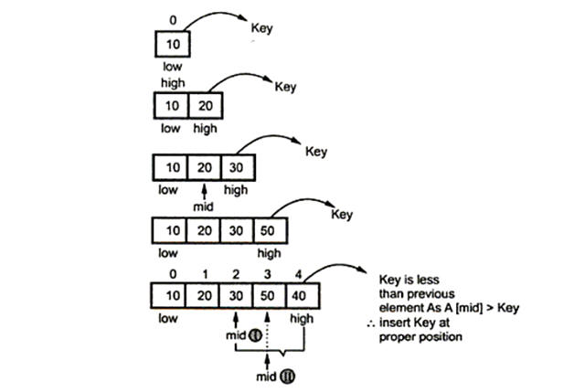
In this method of implementation the sorted sub array is scanned from left to right until the first element greater than or equal to A[n -1] is encountered and then insert A[n -1] right before that element.

10

20

30

50

40

As we get element 40 which is lesser than 50 we will insert 40 before 50. Hence the list will be

10

20

30

40

50

2.

In this method of implementation the sorted sub array is scanned from right to left until the first smaller than or equal to A[n -1] is encountered and then insert A[n -1] right after that element.

10

20

30

50

40

As we get element 50 which is greater than 40 we will insert 50 after 40. Hence the list will be

10

20

30

40

50

This method is also called as straight insertion sort or simply insertion sort.

3.

This third implementation method is called binary insertion sort because in this method the smaller element is searched using binary search method.

For example:

Consider the list of elements to be

10

20

30

50

40

60

Now we will scan the list

Thus after binary insertion sortig method we get a sorted list as,

10

20

30

40

50

60

Let us understand simple insertion sorting method

Example:

Let us consider a list as,

30

70

20

50

40

10

60

The process start with first element

30

70

20

50

40

10

60

Compare 70 with 30 and insert it at its position

30

70

20

50

40

10

60

Compare 20 with the elements in sorted zone and insert it in that zone appropriate position

20

30

70

50

40

10

60

20

30

50

70

40

10

60

20

30

40

50

70

10

60

10

20

30

40

50

70

60

10

20

30

40

50

60

70

Analysis :

Best case:

When the basic operation executed only once then it results in best case time complexity. It happens for almost sorted array. The number of key comparisons can be

Thus average case time complexity of insertion sort is θ(n²).

Worst case:

When the list is sorted in descending order and if we want to sort such a list in ascending order then it results in worst case behavior of algorithm.

1. The basic operation is a key comparison A[ j ] > temp.

2. The basic operation depends upon the size of list i.e. n -1. Hence the basic operation is considered for the range 1 to n -1.

3. The number of key comparisons for such input is

That means worst case time complexity of insertion sort is θ(n²).

Count Sort

The counting sort is not based on comparisons like most sorting methods are. This method of sorting is used when all elements to be sorted fall in a known, finite and reasonably small range.

In Counting sort, we are given array A [1 . . n ] of length n . We required two more arrays, the array B [1 . . n ] holds the sorted output and the array c [1 . . k ] provides temporary working storage.

Example :

Consider an array that we want to sort,

1

4

5

7

2

9

Here the maximum number is 9 so, the other array is created with size of 9. In this array we write the frequencies of numbers or elements.

Now,we create another array that contain the sorted elements.

1^stcalculation :

	1	2	3	4	5	6
B	1

	1	2	3	4	5	6	7	8	9
C’	0	2	2	3	4	4	5	5	6

2^nd calculation :

	1	2	3	4	5	6
B	1		4

	1	2	3	4	5	6	7	8	9
C’	0	2	2	2	4	4	5	5	6

3^rd calculation :

	1	2	3	4	5	6
B	1		4	5

	1	2	3	4	5	6	7	8	9
C’	0	2	2	2	3	4	5	5	6

4^th calculation :

	1	2	3	4	5	6
B	1		4	5	7

	1	2	3	4	5	6	7	8	9
C’	0	2	2	2	3	4	4	5	6

5^th calculation :

	1	2	3	4	5	6
B	1	2	4	5	7

	1	2	3	4	5	6	7	8	9
C’	0	1	2	2	3	4	4	5	6

6^th calculation :

	1	2	3	4	5	6
B	1	2	4	5	7	9

 

	1	2	3	4	5	6	7	8	9
C’	0	1	2	2	3	4	4	5	5

 

Sorted array :

1

2

4

5

7

9

 

Analysis :

The time complexity goes as follows.

time to initialize the array = O(k)

time to read in the numbers and increment the appropriate element of counts= O(n)

time to create the cumulative sum array = O(k)

time to scan read through the list = O(n)

so the total time is,

O(k) + O(n) + O(k) + O(n) = O(k+n)

In practice, we usually use counting sort algorithm when have k = O( n ), in which case running time is O( n ).

Heap and Heap Sort

Heap is a complete binary tree or a almost complete binary tree in which every parent node be either greater or lesser than its child nodes. There are two types of heap which are as follow:

Min Heap :

A min heap is a tree in which value of each node is less than or equal to value of its children nodes.

Max Heap :

A max heap is a tree in which value of each node is greater than or qual to the value of its children nodes.

Parent being greater or lesser in heap is called parental property. Thus heap has two important properties.

1.

It should be a complete binary tree.

2.

It should satisfy parent property.

Before understanding the construction of heap let us learn few basics that are required while constructing heap.

Level of binary tree: the root of the tree is always at level 0. Any node is always at a level one more than its parent nodes level. e.g

Height of the tree: the maximum level is the height of the tree. The height of the tree is also called depth of the tree.e.g. in above diagram the maximum level is 2 hence height of the this tree is 2.

Complete binary tree: the complete binary tree is a binary tree in which all leaves are at the same depth or total number of nodes at each level i are 2ⁱ. e.g.

at level 0→1 node(2ⁱ = 2⁰ = 1)

at level 1→2 node(2ⁱ = 2¹ = 2) and so on.

Almost complete binary tree: the almost complete binary tree is a tree in which:

·

Each node has a left child whenever it has a right child. That means there is always a left child, but for a left child there may not be a right child.

·

The leaf in a tree must be present at height h or h -1. That means all the leaves are on two adjacent levels.

Properties of heap :

There are some important properties that should be followed by heap.

1.

There should be either “complete binary tree” or “almost complete binary tree”.

2.

The root of a heap always contains its largest element.

3.

Each subtree in a heap is also a heap.

Heap Sort :

Heap sort is a sorting method discovered by J. W. J Williams. It works in two stages.

·

Heap construction

·

Deletion of maximum key

Heap construction: First construct a heap for given numbers.

Deletion of maximum key: Delete root key always for (n - 1) times to remaining heap. Hence we will get the elements in decreasing order. For an array implementation of heap, delete the element from heap and put the deleted element in the last position in array. Thus after deleting all the elements one by one, if we collect these deleted elements in an array starting from last index of array.

Example :

Sort the following elements using heap sort

14, 12, 9, 8, 7, 10, 18

Stage 1: heap construction

Stage 2: maximum deletion

Analysis :

As the algorithm works in two stages, we get the running time:

Running time = time required by 1^st stage + time required by 2^nd stage

C(n) = C₁(n) + C₂(n) …(1)

As the heap construction requires O(n) time,

C₁(n) = O(n) …(2)

Now let us compute time required by 2^nd stage.

Let, numbers of key comparisons needed for eliminating root keys from heap are for size from n to 2. Then we can establish following relation.

C₂(n) ≤ 2(n - 1) log₂(n - 1)

But

2(n - 1) log₂(n - 1) = (2n – 2) log₂(n - 1)

2(n - 1) log₂(n - 1) = 2n log₂(n - 1) – 2 log₂(n - 1)

C₂(n) ≤ 2n log₂ n we get,

C₂(n) = O(n log₂ n) …(3)

Now, put equation (2) and (3) in equation (1), we get,

C(n) = O(n) + O(n log₂ n)

C(n) = O(n log₂ n)

Time complexity of heap sort is θ(n log n) in both worst and average case.

Features of heap sort

1.

The time complexity of heap sort is θ(n log n).

2.

This is an in-place sorting. That means it does not require extra storage space while sorting the elements.

3.

For random input it works slower than quick sort.

4.

Heap sort is not a stable sorting method.

5.

The space complexity of heap sort is O(1). As it does not require any extra storage to sort.

Radix Sort

This is a sorting method in which data is sorted by scanning each digit of every element. We sort the list based on least significant bit (LSB) in first pass and then move towards most significant bit (MSB) which results in sorted data.

Example :

Consider following list of elements

25, 37, 18, 82, 55, 64, 78

Phase 1:

8	2
6	4
2	5
5	5
3	7
1	8
7	8

Phase 2:

1	8
2	5
3	7
5	5
6	4
7	8
8	2

Sorted array:

18

25

37

55

64

78

82

Analysis

The running time depends on the stable used as an intermediate sorting algorithm. When each digit is in the range 1 to k , and k is not too large,counting sort is the obvious choice.In case of counting sort, each pass over n d -digit numbers takes O( n + k ) time.

There are d passes, so the total time for Radix sort is θ( n + k ) time. There are d passes, so the total time for Radix sort is θ( dn + kd ). When d is constant then the best and worst case time complexity of radix sort is θ(n).

Bucket Sort

Bucket sort is a technique of sorting the elements with the help of buckets. The buckets are created for sorting the elements with some special data structure called linked list. Like counting sort bucket sort keeps the knowledge of input data.

Example

Sort the following list of elements using bucket sort.

.78, .17, .39, .26, .72, .94, .21, .12, .23, .68

Analysis

If we are using an array of buckets, each item gets mapped to the right bucket in O(1) time, with uniformly distributed keys, the expected number of items per bucket is 1. Thus, sorting each bucket takes O(1) times.

The total effort of bucketing, sorting buckets and concatenating the sorted buckets together is O(n).

 

Chapter 3

Greedy Algorithms

Basics of graphs:

A graph is a collection of vertices or nodes, connected by a collection of edges. Formally graph G is a finite set of (V, E) where V is a set of vertices and E is a set of edges.

Application of graph

· Graph are used in the design of communication and transportation networks, VLSI and other sorts of logic circuits.

· Graphs are used for shape description in computer-aided design and geographic information systems, precedence.

· Graph is used in scheduling systems.

Directed graph

A directed graph G consists of a finite set V-called the vertices or nodes and E set of ordered pairs, called the edges of G.

Undirected graph

A directed graph G consists of a finite set V- set of vertices and E- a set of edges of G.

In a graph, the number of edges coming out of a vertex is called the out-degree of that vertex and the number of edges coming in is called the in-degree. In an undirected graph we just talk about the degree of a vertex as the number of incident edges. By the degree of a graph, we usually mean the maximum degree of its vertices.

Representation of graphs

There are two commonly used methods of representing the graphs.

1. Adjacency matrix

2. Adjacency list

Adjacency matrix:

In this method the graph can be represented by using matrix of n×n such that A[i][j]. if the graph has weights we can store the weights in the matrix.

Adjacency list:

In this method graph can be represented by using linked list. In this method there is an array of linked list for each vertex V in the graph. If the edges have weights then these weights can be stored in the linked list elements.

Now the adjacency matrix of above graph is as follow:

Now the adjacency list of above graph is as follow:

Greedy method

In an algorithmic strategy like Greedy, the decision of solution is taken based on the information available. The greedy method is a straightforward method. This method is popular for obtaining the optimized solutions. In greedy technique, the solution is constructed through a sequence of steps, each expanding a partially constructed solution obtained so far, until a complete solution to the problem is reached. At each step the choice made should be,

Feasible : It should satisfy the problem’s constraints.

Locally optimal : Among all feasible solutions the best choice is to be made.

Irrevocable : Once the particular choice is made then it should not get changed on subsequent steps.

Activities in Greedy method

There are following activities performed in greedy method:

1.

First we select some solution from input domain.

2.

Then we check whether the solution is feasible or not.

3.

From the set of feasible solutions, particular solution that satisfies or nearly satisfies the objective of the function. Such a solution is called optimal solution.

4.

As Greedy method works in stages. At each stage only one input is considered at each time. Based on this input it is decided whether particular input gives the optimal solution or not.

Difference b/w Greedy algorithms and dynamic programming

Greedy method	Dynamic programming
Greedy method is used for obtaining optimum solution.	Dynamic programming is also for obtaining optimum solution.
In greedy method a set of feasible solutions and the picks up the optimum solution.	There is no special set of feasible solutions in this method.
In greedy method the optimum selection is without revising previously generated solutions.	Dynamic programming considers all possible sequences in order to obtain optimum solution.
In greedy method there is no as such guarantee of getting optimum solution.	It is guaranteed that the dynamic programming will generate optimal solution using principle of optimality.

Minimum spanning trees

A spanning tree S is a subset of a tree T in which all the vertices of tree T are present but it may not contain all the edges.

The minimum spanning tree of a weighted connected graph G is called minimum spanning tree if its weight is minimum. There are two spanning tree algorithms:

1.

Prim’s algorithm

2.

Kruskal’s algorithm

Prim’s algorithm

In Prim’s algorithm the pair with the minimum weight is to be chosen. Then adjacent to these vertices whichever is the edge having minimum weight is selected. This process will be continued till all the vertices are not covered. The necessary condition in this case is that the circuit should not be formed.

Example:

Now we construct the tree step by step

Step 1:

Start with vertex a.

Step 2:

Step 3:

Step 4:

Step 5:

Kurskal’s algorithm

In this algorithm the minimum weight is obtained. In this algorithm also the circuit should not be formed. Each time the edge of minimum weight has to be selected, from the graph. It is not necessary in this algorithm to have edges of minimum weights to be adjacent.

Example:

Step 1:

W(a, b) = 1

W(a, c) = 1

W(c, d) = 1

W(c, e) = 1

W(d, e) = 1

W(e, f) = 1

W(a, e) = 2

W(a, f) = 2

W(b, c) = 2

W(b, e) = 2

W(c, i) = 2

W(f, g) = 2

W(a, g) = 3

W(d, i) = 3

W(e, g) = 3

W(e, h) =3

W(e, i) = 3

W(g, h) = 3

W(h, i) = 3

W(g, i) = 5

{a}{b}{c}{d}{e}{f}{g}{h}{i}

Step 2:

{a b}{c}{d}{e}{f}{g}{h}{i}

Step 3:

{a b c}{d}{e}{f}{g}{h}{i}

Step 4:

{a b c d e}{f}{g}{h}{i}

Step 5:

{a b c d e f i}{g}{h}

Step 6:

{a b c d e f g h i}

Huffman’s Codes

Huffman’s coding is a technique for encoding data, by which data compression be done. This technique is used for lossless data compression. This algorithm was developed by David A. Huffman when he was a ph. D student at MIT.

·

In Huffman’s coding method, the data is inputted as a sequence of characters. Then a table of frequency of occurrence of each character in the data is built.

·

From the table of frequencies Huffman’s tree is constructed using Greedy approach.

·

The Huffman’s tree is further used for encoding each character, so that binary encoding is obtained for given data.

·

In Huffman coding there is a specific method of representing each symbol. This method produces a code in such a manner that no code word is prefix of some other code word. Such codes are called prefix codes or prefix free codes. Thus this method is useful for obtaining optimal data compression.

Example:

Let take the string:

“Duke blue devils”

Step 1:

We first to a frequency count of the characters:

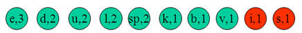
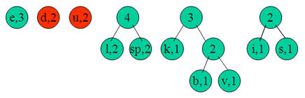
e:3, d:2, u:2, l:2, space:2, k:1, b:1, v:1, i:1, s:1

Step 2:

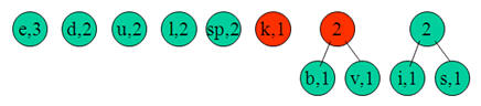
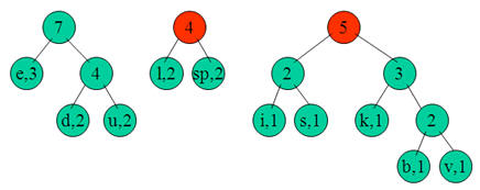
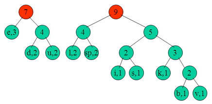
Next we use a Greedy algorithm to build up a Huffman Tree. We take start with nodes for each character.

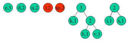
We then pick the nodes with the smallest frequency and combine them together to form a new node.

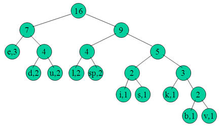
Now we assign codes to the tree by placing a 0 on every left branch and a 1 onevery right branch.

E	00
D	010
U	011
L	100
Sp	101
I	1100
S	1101
K	1110
b	11110
v	11111

These codes are then used to encode the string. Thus, “duke blue devils” turns into:

010 011 1110 00 101 11110 100 011 00 101 010 00 11111 1100 100 1101

Dijkstra’s algorithm

The dijkstra’s algorithm suggests the shortest path from some source node to the some other destination node. The source node or the node from we start measuring the distance is called the start node and the destination node is called the end node. In this algorithm we start finding the distance from the start node and find all the paths from it to neighboring nodes. Among those whichever is the nearest node that path is selected. This process of finding the nearest node is repeated till the end node. Then whichever is the path that path is called the shortest path.

Since in this algorithm all the paths are tried and then we are choosing the shortest path among them, this algorithm is solved by a greedy algorithm. One more thing is that we are having all the vertices in the shortest path and therefore the graph doesn’t give the spanning tree.

Example

P = set which is for nodes which have already selected

T = remaining node

Step 1:

V = a, P = {a} and T = {b, c, d, e, f, z}

Dist (b) = min {old dist (b), dist (a) + w (a, b)}

Dist (b) = min {∞, 0+22} = 22

Dist (c) = min {∞, 0+16} = 16

Dist (d) = min {∞, 0+8} = 8 ← minimum node

Dist (e) = min {∞, 0+ ∞} = ∞

Dist (f) = min {∞, 0+ ∞} = ∞

Dist (z) = min {∞, 0+ ∞} = ∞

Step 2:

V = d, P = {a, d} and T = {b, c, e, f, z}

Dist (b) = min {old dist (b), dist (d) + w (b, d)}

Dist (b) = min {22, 8 + ∞} = 22

Dist (c) = min {16, 8 + 10} = 16

Dist (e) = min {∞, 8 + ∞} = ∞

Dist (f) = min {∞, 8 + 6} = 14 ← minimum node

Dist (z) = min {∞, 8 + ∞} = ∞

Step 3:

V = f, P = {a, d, f} and T = {b, c, e, z}

Dist (b) = min {old dist (b), dist (f) + w (f, b)}

Dist (b) = min {22, 14 + 7} = 21

Dist (c) = min {16, 14 + 3} = 16 ← minimum node

Dist (e) = min {∞, 14 + ∞} = ∞

Dist (z) = min {∞, 14 + 9} = 23

Step 4:

V= c, P = {a, d, f, c}andT = {b, e, z}

Dist (b) = min {21, 16 + 20} = 21

Dist (e) = min {∞, 16 + 4} = 20 ← minimum node

Dist (z) = min {23, 16 + 10} = 23

Step 5:

V = e, P = {a, d, f, c, e} and T = {b, z}

Dist (b) = min {21, 20 + 2} = 21← minimum node

Dist (z) = min {23, 20 + 4} = 23

Step 6:

V = b, P = {a, d, f, c, e, b} and T = {z}

Dist (z) = min {23, 21 + 2} = 23

Now the target vertex for finding the shortest path is z. hence the length of the shortest path from the vertex a - z is 23. The shortest path is as follow:

Chapter 4

Dynamic Programming

Dynamic Programming

Dynamic programming is typically applied to optimization problem. This technique is invented by a U.S Mathematician Richard Bellman in 1950. In the word dynamic programming the word programming stands for planning and it does not mean by computer programming.

·

Dynamic programming is a technique for solving problems with overlapping subproblems.

·

In this method each subproblem is solved only once. The result of each subproblem is recorded in a table from which we can obtain a solution to the original problem.

Steps of Dynamic Programming

Dynamic programming design involves 4 major steps:

1.

Characterize the structure of optimal solution. That means develop a mathematical notation that can express any solution and subsolution for the given problem.

2.

Recursively define the value of an optimal solution.

3.

By using bottom up technique compute value of optimal solution. For that you have to develop a recurrence relation that relates a solution to its subsolutions, using the mathematical notation of step 1.

4.

Compute an optimal solution from computed information.

Warshall Algorithm

The Warshall algorithm, actually called as Floyd Warshall algorithm is for finding the shortest path between every pair of vertices in the graph. This algorithm works for both directed as well as undirected graphs. This algorithm is invented by Robert Floyd and Stephen Warshall hence it is often called as Floyd Warshall algorithm.

		D(0)							R(0)
	A	M	L	B	X			A	M	L	B	X
A	∞	23	10	∞	18		A	1	2	3	4	5
M	23	∞	10	48	∞		M	1	2	3	4	5
L	10	10	∞	19	7		L	1	2	3	4	5
B	∞	48	19	∞	20		B	1	2	3	4	5
X	18	∞	7	20	∞		X	1	2	3	4	5

 

 

		D(0)							R(0)
	A	M	L	B	X			A	M	L	B	X
A	∞	23	10	∞	18		A	1	2	3	4	5
M	23	∞	10	48	∞		M	1	2	3	4	5
L	10	10	∞	19	7		L	1	2	3	4	5
B	∞	48	19	∞	20		B	1	2	3	4	5
X	18	∞	7	20	∞		X	1	2	3	4	5

 

		D(0)							R(0)
	A	M	L	B	X			A	M	L	B	X
A	∞	23	10	∞	18		A	1	2	3	4	5
M	23	∞	10	48	∞		M	1	2	3	4	5
L	10	10	∞	19	7		L	1	2	3	4	5
B	∞	48	19	∞	20		B	1	2	3	4	5
X	18	∞	7	20	∞		X	1	2	3	4	5

		D(0)							R(0)
	A	M	L	B	X			A	M	L	B	X
A	∞	23	10	∞	18		A	1	2	3	4	5
M	23	46	10	48	∞		M	1	1	3	4	5
L	10	10	∞	19	7		L	1	2	3	4	5
B	∞	48	19	∞	20		B	1	2	3	4	5
X	18	∞	7	20	∞		X	1	2	3	4	5

		D(0)							R(0)
	A	M	L	B	X			A	M	L	B	X
A	∞	23	10	∞	18		A	1	2	3	4	5
M	23	46	10	48	∞		M	1	1	3	4	5
L	10	10	∞	19	7		L	1	2	3	4	5
B	∞	48	19	∞	20		B	1	2	3	4	5
X	18	∞	7	20	∞		X	1	2	3	4	5

		D(0)							R(0)
	A	M	L	B	X			A	M	L	B	X
A	∞	23	10	∞	18		A	1	2	3	4	5
M	23	46	10	48	∞		M	1	1	3	4	5
L	10	10	∞	19	7		L	1	2	3	4	5
B	∞	48	19	∞	20		B	1	2	3	4	5
X	18	∞	7	20	∞		X	1	2	3	4	5

		D(0)							R(0)
	A	M	L	B	X			A	M	L	B	X
A	∞	23	10	∞	18		A	1	2	3	4	5
M	23	46	10	48	∞		M	1	1	3	4	5
L	10	10	∞	19	7		L	1	2	3	4	5
B	∞	48	19	∞	20		B	1	2	3	4	5
X	18	∞	7	20	∞		X	1	2	3	4	5

		D(0)							R(0)
	A	M	L	B	X			A	M	L	B	X
A	∞	23	10	∞	18		A	1	2	3	4	5
M	23	46	10	48	41		M	1	1	3	4	1
L	10	10	∞	19	7		L	1	2	3	4	5
B	∞	48	19	∞	20		B	1	2	3	4	5
X	18	∞	7	20	∞		X	1	2	3	4	5

		D(0)							R(0)
	A	M	L	B	X			A	M	L	B	X
A	∞	23	10	∞	18		A	1	2	3	4	5
M	23	46	10	48	41		M	1	1	3	4	1
L	10	10	∞	19	7		L	1	2	3	4	5
B	∞	48	19	∞	20		B	1	2	3	4	5
X	18	∞	7	20	∞		X	1	2	3	4	5

		D(0)							R(0)
	A	M	L	B	X			A	M	L	B	X
A	∞	23	10	∞	18		A	1	2	3	4	5
M	23	46	10	48	41		M	1	1	3	4	1
L	10	10	∞	19	7		L	1	2	3	4	5
B	∞	48	19	∞	20		B	1	2	3	4	5
X	18	∞	7	20	∞		X	1	2	3	4	5

 

		D(0)							R(0)
	A	M	L	B	X			A	M	L	B	X
A	∞	23	10	∞	18		A	1	2	3	4	5
M	23	46	10	48	41		M	1	1	3	4	1
L	10	10	20	19	7		L	1	2	1	4	5
B	∞	48	19	∞	20		B	1	2	3	4	5
X	18	∞	7	20	∞		X	1	2	3	4	5

		D(0)							R(0)
	A	M	L	B	X			A	M	L	B	X
A	∞	23	10	∞	18		A	1	2	3	4	5
M	23	46	10	48	41		M	1	1	3	4	1
L	10	10	20	19	7		L	1	2	1	4	5
B	∞	48	19	∞	20		B	1	2	3	4	5
X	18	∞	7	20	∞		X	1	2	3	4	5

		D(0)							R(0)
	A	M	L	B	X			A	M	L	B	X
A	∞	23	10	∞	18		A	1	2	3	4	5
M	23	46	10	48	41		M	1	1	3	4	1
L	10	10	20	19	7		L	1	2	1	4	5
B	∞	48	19	∞	20		B	1	2	3	4	5
X	18	∞	7	20	∞		X	1	2	3	4	5

		D(0)							R(0)
	A	M	L	B	X			A	M	L	B	X
A	∞	23	10	∞	18		A	1	2	3	4	5
M	23	46	10	48	41		M	1	1	3	4	1
L	10	10	20	19	7		L	1	2	1	4	5
B	∞	48	19	∞	20		B	1	2	3	4	5
X	18	∞	7	20	∞		X	1	2	3	4	5

		D(0)							R(0)
	A	M	L	B	X			A	M	L	B	X
A	∞	23	10	∞	18		A	1	2	3	4	5
M	23	46	10	48	41		M	1	1	3	4	1
L	10	10	20	19	7		L	1	2	1	4	5
B	∞	48	19	∞	20		B	1	2	3	4	5
X	18	∞	7	20	∞		X	1	2	3	4	5

		D(0)							R(0)
	A	M	L	B	X			A	M	L	B	X
A	∞	23	10	∞	18		A	1	2	3	4	5
M	23	46	10	48	41		M	1	1	3	4	1
L	10	10	20	19	7		L	1	2	1	4	5
B	∞	48	19	∞	20		B	1	2	3	4	5
X	18	∞	7	20	∞		X	1	2	3	4	5

		D(0)							R(0)
	A	M	L	B	X			A	M	L	B	X
A	∞	23	10	∞	18		A	1	2	3	4	5
M	23	46	10	48	41		M	1	1	3	4	1
L	10	10	20	19	7		L	1	2	1	4	5
B	∞	48	19	∞	20		B	1	2	3	4	5
X	18	∞	7	20	∞		X	1	2	3	4	5

		D(0)							R(0)
	A	M	L	B	X			A	M	L	B	X
A	∞	23	10	∞	18		A	1	2	3	4	5
M	23	46	10	48	41		M	1	1	3	4	1
L	10	10	20	19	7		L	1	2	1	4	5
B	∞	48	19	∞	20		B	1	2	3	4	5
X	18	∞	7	20	∞		X	1	2	3	4	5

		D(0)							R(0)
	A	M	L	B	X			A	M	L	B	X
A	∞	23	10	∞	18		A	1	2	3	4	5
M	23	46	10	48	41		M	1	1	3	4	1
L	10	10	20	19	7		L	1	2	1	4	5
B	∞	48	19	∞	20		B	1	2	3	4	5
X	18	41	7	20	∞		X	1	1	3	4	5

		D(0)							R(0)
	A	M	L	B	X			A	M	L	B	X
A	∞	23	10	∞	18		A	1	2	3	4	5
M	23	46	10	48	41		M	1	1	3	4	1
L	10	10	20	19	7		L	1	2	1	4	5
B	∞	48	19	∞	20		B	1	2	3	4	5
X	18	41	7	20	∞		X	1	1	3	4	5

		D(0)							R(0)
	A	M	L	B	X			A	M	L	B	X
A	∞	23	10	∞	18		A	1	2	3	4	5
M	23	46	10	48	41		M	1	1	3	4	1
L	10	10	20	19	7		L	1	2	1	4	5
B	∞	48	19	∞	20		B	1	2	3	4	5
X	18	41	7	20	∞		X	1	1	3	4	5

		D(0)							R(0)
	A	M	L	B	X			A	M	L	B	X
A	∞	23	10	∞	18		A	1	2	3	4	5
M	23	46	10	48	41		M	1	1	3	4	1
L	10	10	20	19	7		L	1	2	1	4	5
B	∞	48	19	∞	20		B	1	2	3	4	5
X	18	41	7	20	∞		X	1	1	3	4	5

		D(0)							R(0)
	A	M	L	B	X			A	M	L	B	X
A	∞	23	10	∞	18		A	1	2	3	4	5
M	23	46	10	48	41		M	1	1	3	4	1
L	10	10	20	19	7		L	1	2	1	4	5
B	∞	48	19	∞	20		B	1	2	3	4	5
X	18	41	7	20	36		X	1	2	3	4	1

 

		D(1)							R(1)
	A	M	L	B	X			A	M	L	B	X
A	∞	23	10	∞	18		A	1	2	3	4	5
M	23	46	10	48	41		M	1	1	3	4	1
L	10	10	20	19	7		L	1	2	1	4	5
B	∞	48	19	∞	20		B	1	2	3	4	5
X	18	41	7	20	36		X	1	2	3	4	1

 

		D(1)							R(1)
	A	M	L	B	X			A	M	L	B	X
A	∞	23	10	∞	18		A	1	2	3	4	5
M	23	46	10	48	41		M	1	1	3	4	1
L	10	10	20	19	7		L	1	2	1	4	5
B	∞	48	19	∞	20		B	1	2	3	4	5
X	18	41	7	20	36		X	1	2	3	4	1

 

		D(1)							R(1)
	A	M	L	B	X			A	M	L	B	X
A	46	23	10	71	18		A	2	2	3	2	5
M	23	46	10	48	41		M	1	1	3	4	1
L	10	10	20	19	7		L	1	2	1	4	5
B	71	48	19	96	20		B	2	2	3	2	5
X	18	41	7	20	36		X	1	2	3	4	1

 

		D(2)							R(2)
	A	M	L	B	X			A	M	L	B	X
A	46	23	10	71	18		A	2	2	3	2	5
M	23	46	10	48	41		M	1	1	3	4	1
L	10	10	20	19	7		L	1	2	1	4	5
B	71	48	19	96	20		B	2	2	3	2	5
X	18	41	7	20	36		X	1	2	3	4	1

		D(2)							R(2)
	A	M	L	B	X			A	M	L	B	X
A	46	23	10	71	18		A	2	2	3	2	5
M	23	46	10	48	41		M	1	1	3	4	1
L	10	10	20	19	7		L	1	2	1	4	5
B	71	48	19	96	20		B	2	2	3	2	5
X	18	41	7	20	36		X	1	2	3	4	1

		D(2)							R(2)
	A	M	L	B	X			A	M	L	B	X
A	20	20	10	29	17		A	3	3	3	3	3
M	20	20	10	29	17		M	3	3	3	3	3
L	10	10	20	19	7		L	1	2	1	4	5
B	29	29	19	38	20		B	3	3	3	3	5
X	17	17	7	20	14		X	3	3	3	4	3

		D(3)							R(3)
	A	M	L	B	X			A	M	L	B	X
A	20	20	10	29	17		A	3	3	3	3	3
M	20	20	10	29	17		M	3	3	3	3	3
L	10	10	20	19	7		L	1	2	1	4	5
B	29	29	19	38	20		B	3	3	3	3	5
X	17	17	7	20	14		X	3	3	3	4	3

		D(3)							R(3)
	A	M	L	B	X			A	M	L	B	X
A	20	20	10	29	17		A	3	3	3	3	3
M	20	20	10	29	17		M	3	3	3	3	3
L	10	10	20	19	7		L	1	2	1	4	5
B	29	29	19	38	20		B	3	3	3	3	5
X	17	17	7	20	14		X	3	3	3	4	3

		D(4)							R(4)
	A	M	L	B	X			A	M	L	B	X
A	20	20	10	29	17		A	3	3	3	3	3
M	20	20	10	29	17		M	3	3	3	3	3
L	10	10	20	19	7		L	1	2	1	4	5
B	29	29	19	38	20		B	3	3	3	3	5
X	17	17	7	20	14		X	3	3	3	4	3

		D(4)							R(4)
	A	M	L	B	X			A	M	L	B	X
A	20	20	10	29	17		A	3	3	3	3	3
M	20	20	10	29	17		M	3	3	3	3	3
L	10	10	20	19	7		L	1	2	1	4	5
B	29	29	19	38	20		B	3	3	3	3	5
X	17	17	7	20	14		X	3	3	3	4	3

		D(4)							R(4)
	A	M	L	B	X			A	M	L	B	X
A	20	20	10	29	17		A	3	3	3	3	3
M	20	20	10	29	17		M	3	3	3	3	3
L	10	10	14	19	7		L	1	2	5	4	5
B	29	29	19	38	20		B	3	3	3	3	5
X	17	17	7	20	14		X	3	3	3	4	3

		D(5)							R(5)
	A	M	L	B	X			A	M	L	B	X
A	20	20	10	29	17		A	3	3	3	3	3
M	20	20	10	29	17		M	3	3	3	3	3
L	10	10	14	19	7		L	1	2	5	4	5
B	29	29	19	38	20		B	3	3	3	3	5
X	17	17	7	20	14		X	3	3	3	4	3

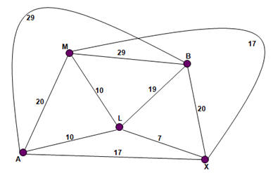
Chapter 5

String Matching

Introduction

String matching is a very important subject in the wider domain of text processing. String matching algorithms are basic components used in implementation of practical softwares existing under most operating systems. Moreover, they emphasize programming methods that serve as paradigms in other fields of computer science such as system programming or software design. In string matching algorithms data is memorized in various ways.

Pattern matching

A string is a sequence of characters. Let text[0,…, n-1] be the string of length n, and pattern[0,…, m-1] be some substring of length m, then pattern matching is a technique of finding the substring in text which is equal to pattern. The pattern matching problem is also called as PMP.

Applications of pattern matching

1.

Pattern matching technique is used in text editors.

2.

Search engines use the pattern matching algorithm for matching the query submitted by the user.

3.

In biological research pattern matching algorithm is used.

Pattern matching algorithm

There are various algorithm used to implement the pattern matching problem. Some of them are:

1.

Knuth- Morris- Pratt

2.

Boyer- Moore

Knuth- Morris- Pratt’s algorithm

Knuth-Morris-Pratt’s algorithm compares the text with pattern in left to right. But in this algorithm shift is made more intelligently if match is not found. The shift distance is determined by the widest border of matching prefix of P.

Symbol from 0 to 4 are matched. But the symbols at position 5 are not matching. The shift distance is determined by the widest border of matching prefix P. The matching prefix is abcab, assume it to be m.

The widest border is ab with width b = 2. Hence shift distance is m – b = 5 – 2 = 3. Hence the comparison is made.

Example

The KMP algorithm makes use of information gained by previous symbol comparisons. It never re-compares a text symbol that has matched a pattern symbol. Hence time complexity of KMP algorithm is O(n).

Boyer – Moore’s algorithm

This algorithm works on two ideas

1.

Comparing the pattern with text from right to left.

2.

The shift size can be computed using two tables, bad symbol table and good suffix table.

Bad symbol shift:

When mismatch occurs then this idea is used. How much is to be shifted – is decided by using bad symbol shift, which is basically based on mismatch that occurs on text’s character.

·

If the rightmost character of the pattern does not match then shift the pattern to the right by pattern’s length.

·

If the rightmost character of pattern matched with the text, then move from right to left and compare each character with text. If at some point a mismatch text’s character ‘T’ occurs after k matches (when k > 0) then first build the shift table. And then compute bad symbol shift.

Let us first understand the procedure for building shift table. Following are the two steps used to compute shift table.

1.

If ‘T’ is not among first m – 1 characters of pattern then

Table (T) = the pattern length m

2.

Otherwise

Table (T) = the distance from the rightmost T among first m – 1 characters of patterns to its last character.

For example

For a word RADAR the length of this pattern is 5. Hence all the entries of each alphabet except R, A, D will be filled up by 5.

Now,

If we scan from right to left then character A appears at position 1. Hence make entry for alphabet A as 1.

D occurs at position 2. Hence make entry for D as 2 in the shift table.

Since R appears at position 4. Make the entry 4 in shift table for R.

The shift table for pattern RADAR would be

After building the shift table, the bad symbol shift can be computed. It is denoted by d₁.

d₁ = max {text (T) – k, 1}

For example

If we want to search for the pattern EVENING from given text then we construct shift table first as

Then,

Master Theorem

The master theorem equation is as follow:

T(n) = a T(n/b) + n^d

The master theorem is

If f(n) є θ(n^d) then

1. T(n) = θ(n^d) if a< b^d

2. T(n) = θ(n^d log n) if a= b^d

3. T(n) = θ(n^log_b^a) if a> b^d

Another variation of Master theorem is

For T(n) = aT(n/b) + f(n) if n ≥ d

1. If f(n) is O(n^log_b^{a - є}), then T(n) = θ(n^log_b^a)

2. If f(n) is θ(n^log_b^a log^kn), then T(n) = θ(n^log_b^a log^k+1 n)

3. If f(n) is Ω(n^log_b^a+є), then T(n) = θ(f(n))

Example 1 :

T (n) = 3T (n/2) + n²

Here a = 3, b = 2 and f(n) = n²

n^log_b^a = n^log₂³

n^log_b^a = n^1.58

Now n²> n^1.58

f(n) > n^log_b^a

Hence by case 3 of master theorem

T(n) = θ(n²)

Example 2 :

T(n) = 4T(n/2) + n²

Here a = 4, b = 2 and f(n) = n²

n^log_b^a = n^log₂⁴

n^log_b^a = n²

Now n² = n²

f(n) = n^log_b^a

It is case 2 of the master theorem

T(n) = θ(n^d log n)

T(n) = θ(n² log n)

Example 3 :

T(n) = T(n/2) + 2ⁿ

Here a = 1, b = 2 and f(n) = 2ⁿ

n^log_b^a = n^log₂¹

n^log_b^a = n

from above value it is clear that

f(n) > n^log_b^a

Hence by case 3 of master theorem

T(n) = θ(f(n))

T(n) = θ(2ⁿ)

Example 4 :

T(n) = 2ⁿ T(n/2) + nⁿ

Here a = 2ⁿ, b = 2 and f(n) = nⁿ

Since a is not constant therefore it cannot be solved by master theorem.

Example 5 :

T(n) = 16T(n/4) + n

Here a = 16, b = 4 and f(n) = n

n^log_b^a = n^log₄¹⁶

n^log_b^a = n²

Now n²> n therefore

f(n) < n^log_b^a

Hence by case 1 of master theorem

T(n) = θ(n²)

Example 6 :

T(n) = 2T(n/2) + n log n

Here a = 2, b = 2 and f(n) = n log n

n^log_b^a = n^log₂²

n^log_b^a = n¹

n^log_b^a = n

Since f(n) = n log n

And n^log_b^a = n

Therefore f(n) and n^log_b^a has same rate of growth, therefore it is case 2 of master theorem

T(n) = θ(n^log_b^a log^k+1 n)

T(n) = θ(n log² n)

Example 7 :

T(n) = 2T(n/2) + n/log n

Here a = 2, b = 2 and f(n) = n/log n

Since f(n) is not polynomial, therefore master theorem does not apply.

Example 8 :

T(n) = 2T(n/4) + n^0.51

Here a = 2, b = 4 and f(n) = n^0.51

n^log_b^a = n^log₄²

n^log_b^a = n^0.5

n^0.51> n^0.5

f(n) > n^log_b^a

Hence by case 3 of master theorem

T(n) = θ(f(n))

T(n) = θ(n^0.51)

Example 9 :

T(n) = 0.5T(n/2) + 1/n

Here a = 0.5, b = 2 and f(n) = 1/n

Since a < 1, therefore master theorem does not apply.

Example 10 :

T(n) = 16T(n/4) + n!

Here a = 16, b = 4 and f(n) = n!

n^log_b^a = n^log₄¹⁶

n^log_b^a = n²

n! > n²

f(n) > n^log_b^a

Hence by case 3 of master theorem

T(n) = θ(f(n))

T(n) = θ(n!)

Example 11 :

T(n) = 3T(n/2) + n

Here a = 3, b = 2 and f(n) = n

n^log_b^a = n^log₂³

n^log_b^a = n^1.58

n < n^1.58

f(n) < n^log_b^a

Hence by case 1 of master theorem

T(n) = θ(n^1.58)

Example 12 :

T(n) = 4T(n/2) + cn

Here a = 4, b = 2 and f(n) = cn

n^log_b^a = n^log₂⁴

n^log_b^a = n²

cn < n²

f(n) < n^log_b^a

Hence by case 1 of master theorem

T(n) = θ(n²)

Example 13 :

T(n) = 3T(n/4) + n log n

Here a = 3, b = 4 and f(n) = n log n

n^log_b^a = nlog ₄³

n^log_b^a = n^0.79

n log n > n^0.79

f(n) > n^log_b^a

Hence by case 3 of master theorem

T(n) = θ(n log n)

Example 14 :

T(n) = 3T(n/3) + n^1/2

Here a = 3, b = 3 and f(n) = n^1/2

n^log_b^a = n^log₃³

n^log_b^a = n¹

n^1/2> n

f(n) < n^log_b^a

Hence by case 1 of master theorem

T(n) = θ(n)