MS Excel Tutorial About VLOOKUP
VLOOKUP Function In MS Excel
The Excel VLOOKUP function is used when we want to search the value in one column (left most column) and return (display) the value form other column from the same row. in simple word we say that VLOOKUP function is used for a vertical lookup for the purpose of searching for a value in the left-most column of table and return a value from the same row in the index number position. where index number is the column number from which result display.
Now we explain Excel VLOOKUP function with syntax and examples.
The syntax of the function is :
VLOOKUP( value, table_array, index_number, [not_exact_match] )
where value is the searched value. Table array is range (one or more then one column where data is store ) and index number is column from which result will be display
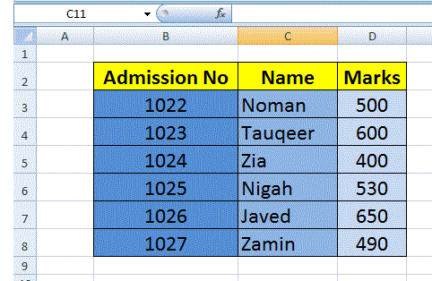
we explain this with an example if we have data as given in following table:

If we want to found the Name of any student by giving Admission Number . For example if we give the admission no 1025 and set index as column 2 which is name column then it return Zia.
syntax as under:
=VLOOKUP( 1024 , B2:D8 , 2 )
Result display ' Zia '
we take a detail look

According to above picture
-
First Select the Cell Where you want to display the result . in My case C12
-
Select Formulas Menu and Click on Insert Function and select the Lookup and references function and then VLOOKUP function Form Category List.

Enter Lookup value C11 where we write the Admission Number for searching, Table array B2:B8 and Col_Index 2 .

Click on Ok Button.
Now write any admission Number in C11 cell then VLOOKUP function return The name of That admission number in C12.

we also write the function in the Cell where we want to calculate. as given below
=VLOOKUP( C11 , B2:D8 , 2 )
PMT() Financial Functions
Calculate the Sum of a Range Using AutoSum function
User Define Function (UDF) In Excel
Macros In Excel
Relative and Absolute Cell Reference in MS Excel
Page Setting and printing In MS Excel
Fill In Excel
How we use The Functions in MS Excel
How we Write Excel Formulas
Components of Excel 2007 Environment
Rounding The Numbers MS Excel
SUMIF FUNCTION In MS EXCEL
COUNTIF Function In MS Excel
COUNTBLANK Function In MS Excel
VLOOKUP Function In MS Excel
Pivot Table In MS Excel
Consolidation In MS Excel
Remove Duplicate Value In MS Excel
Convert Excel Data in to a Table